Disclaimer: This post is about one of proj-h’s live trading strategy. You can check out details about the performance of the strategy here

In the last blog post we described the technical foundation that proj-h is build on, but the even best trading platform is useless without some algorithms running on it. Hence in the last months the main focus of the project has been on getting some trading going and some relatively simple algorithms have been implemented. One of those strategies is the classical Bollinger Bands that I want to describe in some detail in this Blog post. Some of you might now be thinking “Oh my god, Bollinger Bands, I’ve landed in quant trading kindergarden” and well, you are right, as proj-h is also here for education. But more importantly, the reason for this choice is that the main goal of having this algo running is not to make money (and don’t fret, as of now the strategy didn’t), but to validate the trading platform. Anyhow, I still think it makes sense to describe the idea behind the algorithm, the mathematical foundation, its strengths, weaknesses and the detailed implementation in proj-h.

How do Bollinger Bands work?

Bollinger Bands is pretty much the poster child of a whole family of trading algorithms, mean reversion. The idea behind mean reversion is, that while there are larger up and down movements in a market, in the short term prices typically oscillate around a given current level. In simple terms, what goes up must come down and what goes down eventually comes up again. While this would be a good fortune cookie quote, we need a bit more to go on to make a trading strategy out of it.

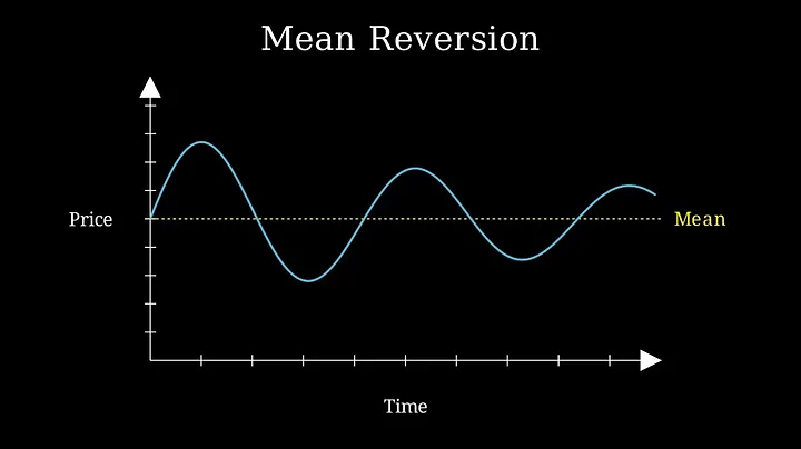
Bollinger Bands translates this simple principle into an algorithm by using two mathematical methods to determine what the current “normal” price level is and what counts as high and low prices: SMA (simple moving average) and standard deviation. First, a time window is defined that the strategy should look at. This is a strategy parameter and needs to be defined by the trader using back-testing, optimization, gut feeling or a magic 8 ball. Then, all trade events (this could be either trades or any abstraction of them like bars) in this the time window are collected and the mean price is calculated, which is the same as calculating the SMA. The same trades are then used to calculate the standard deviation of the time window. We use the standard deviation as measurement for the current volatility of the market, so a low standard deviation means that the market trades very close around the mean, while a large one indicates a wild market with big price swings. These two values are then used to calculate three bands (hence the name of the strategy), the upper band, which is the SMA + standard deviation * x, the middle band, which is simply the SMA, and the lower band, which is the SMA + standard deviation * x.

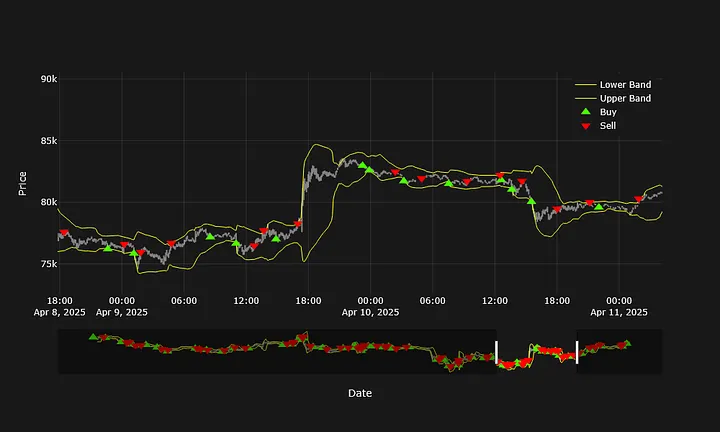
Now that we calculated upper, middle and lower band, the logic of the algorithm is pretty simple. If the current price on the market is above the upper band, we want to place a sell order, as the theory behind the algorithm says that the prices are abnormally high and should return to the mean. Once the short position is opened, we wait until the prices hit the middle band again and then close the position (hopefully in the money). Vice versa, if the price moves below the lower band, we want to open a long position, which then will be closed when prices hit the middle band again.

As the attentive reader that you are you surely have realized the introduction of a new variable, x. x is the second (and last) parameter, that the Bollinger Band strategy employs, which indicates the aggressiveness of the strategy. A higher x leads to a greater the distance between the SMA and upper and lower bands, which leads to less trades that in theory should have a greater probability to be successful.

As a short side note, in quantitative trading when calculating mean prices or standard deviations, one should always calculate the volume weighted mean, also taking into account the traded quantities. Otherwise a very small trade has the same influence on the mean for a given time window as a very large one.

Strengths of the Bollinger Bands strategy

Every strategy has it’s strengths and weaknesses, even the mighty Bollinger Bands. Lets have a look at it’s advantages.

Simplicity

As you might have noticed, the strategy is really simple, which in my opinion has a certain elegance. It is easy to understand to idea behind it and it makes sense why it should work, as markets will always go up and down to a certain degree (if you know a market that only goes up, please let me know though). So it just makes intuitive sense, that a well parameterized Bollinger Bands strategy could make money.

Adaptability

By using information deprived directly from the market it is trading in, the strategy adapts to current conditions by making the bands narrower or wider. This “auto-adaptability” is a great feature for any strategy to have, as it simply makes the strategy more widely applicable.

Clear Signals

Bollinger Bands offer defined levels for potential action. Crossing the upper band is a clear signal to consider shorting, crossing the lower band suggests looking for a long entry, and the middle band provides a logical (though not always optimal) target. This goes together with the simplicity point, in that it is relatively clear how to implement this strategy, which is possible without an elaborate position opening/closing logic in the algorithm itself.

Weaknesses of the Bollinger Bands strategy

Except Arnold Schwarzenegger, most things in life also have some weaknesses. While simple and adaptable, Bollinger Bands are far from a holy grail (spoiler alert: no trading strategy is).

The Trend is NOT Your Friend (here)

Bollinger Bands are built on the idea of mean reversion, so prices bouncing back towards the mean. What happens when it catches a strong, persistent trend upwards or downwards? Utter Disaster. In a strong uptrend, the strategy would open a short once the upper band is hit and then wave goodbye at any profit as it watches the position move more on more out of the money (this article was written on the 12th of April, so talking about strong trends I am looking in your direction Donald).

Lagging Behind the Action

Remember, the bands are calculated using the data in the selected time window, which means they are inherently lagging indicators. They tell you what the average price and volatility have been, not what they will be. So while all the actions the strategy takes would have worked wonderfully in the past, there is no guarantee that they will also work out in the future.

Parameter Puzzle

The strategy's effectiveness hinges heavily on the two parameters: the lookback period and the multiplier 'x'. Choosing the right combination is crucial, but it's not straightforward. A setting that works beautifully on one market or even one day, might be terrible on another. Finding good parameters requires diligent backtesting and optimization, but even then, parameters optimized for past performance are no guarantee of future success (hello, overfitting!). We will discuss this topic in depth in another blog post.

proj-h’s implementation of the strategy

There is always some wiggle room with the implementation of a trading strategy. So while it is in theory pretty clear, what the algorithm should do, no two algo codes will ever be the same. Hence, here is a exact description of how Bollinger Bands work in the world of proj-h currently.

Initialization

First off, when the strategy spins up, it is establishing a baseline position. If the strategy hasn't done this yet and has cash available, it places a buy order for roughly half its budget's worth of the asset. This is a one-time action to get the strategy invested from the start. The reason for this implementation is, that at the moment naked shorts are actually not possible. So to enable some form of going short, a baseline position is required and being short actually means being flat.

Core Logic

With each new trade event, the price and timestamp are added to a rolling history. The strategy keeps this history trimmed to a specific time window. If a price point is older than this window, it gets dropped. Before doing any calculations, it checks if it actually has enough data covering the required time window. If not, it waits for more data.

Once there's sufficient history, it calculates the Simple Moving Average (SMA) and the Standard Deviation using only the prices within the current time window. These are then used to compute the upper band (SMA + multiplier * StdDev) and lower band (SMA - multiplier * StdDev).

Here's where the trading logic comes in:

1. Price Drops Below Lower Band: If the price crosses below the lower band and the strategy isn't already holding a long position (and didn't just hit the lower band), it signals a buy. It first cancels any existing open orders, recalculates its available cash, and then places a limit buy order for its entire available cash balance, slightly above the current price.
2. Price Rises Above Upper Band: Conversely, if the price pops above the upper band and the strategy isn't already effectively short (meaning, holding mostly cash) and didn't just hit the upper band, it's a sell signal. Again, it cancels open orders, figures out the total quantity of the asset it holds, and places a limit sell order for that entire quantity, slightly below the current price.
3. Returning to the Middle (from Long): If the strategy is currently long and the price climbs back up to the SMA (the middle band), it aims to return to its baseline. It cancels orders, calculates the quantity it holds, and then sells off a portion (specifically, 1 minus the baseline percentage – so 50% in the default case) of its holdings. The sell order is placed slightly below the current price.
4. Returning to the Middle (from Short): If the strategy is short (meaning it sold everything) and the price falls back down to the SMA, it aims to re-buy its baseline position. It cancels orders, calculates its available cash, and places a limit buy order for an amount equivalent to its target baseline percentage of its capital, slightly above the current price.
5. Inside the Bands: If the price is simply meandering between the upper and lower bands, the strategy resets the flags that track whether the bands were recently hit, preparing for the next potential breakout.

Finally, for operational purposes, the strategy periodically logs the calculated band values and recent price statistics (close, high, low) to a database. When the trading session ends, there's a cleanup phase: it processes any final order fills, cancels all remaining open orders, and places orders to close out any remaining long or short position entirely, effectively flattening its book.

Conclusion

So now that you learned a bunch about Bollinger Bands you can check out it’s current performance here. Like mentioned in the intro, the goal of the implementation is way more to test the technical platform and it has helped tremendously to iron out some of the kinks that come with having a live software running. In the next blog post, we will have a closer look at the arch enemy of mean reversion, trend following, and after we will turn our attention to juicier topics like the complete validation of trading platforms.

If you have read this far, you are a true hero and I can not thank you enough. As always, any feedback is welcome, so don't hesitate to shoot me a message at hello@proj-h.com or DM me on LinkedIn or on our newest channel, Instagram.